Independent Alleles solved by 6595

Mendel's Second Law

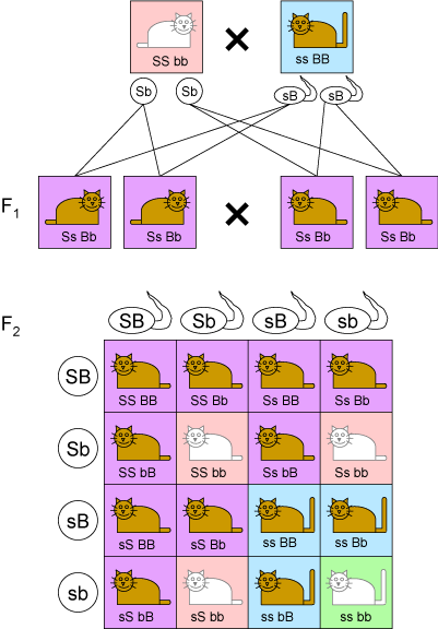
Figure 1. Mendel's second law dictates that every one of the 16 possible assignments of parental alleles is equally likely. The Punnett square for two factors therefore places each of these assignments in a cell of a 4 X 4 table. The probability of an offspring's genome is equal to the number of times it appears in the table, divided by 16.

Recall that Mendel's first law states that for any factor, an individual randomly assigns one of its two alleles to its offspring. Yet this law does not state anything regarding the relationship with which alleles for different factors will be inherited.

After recording the results of crossing thousands of pea plants for seven years, Mendel surmised that alleles for different factors are inherited with no dependence on each other. This statement has become his second law, also known as the law of independent assortment.

What does it mean for factors to be "assorted independently?" If we cross two organisms, then a shortened form of independent assortment states that if we look only at organisms having the same alleles for one factor, then the inheritance of another factor should not change.

For example, Mendel's first law states that if we cross two $\textrm{Aa}$ organisms, then 1/4 of their offspring will be $\textrm{aa}$, 1/4 will be $\textrm{AA}$, and 1/2 will be $\textrm{Aa}$. Now, say that we cross plants that are both heterozygous for two factors, so that both of their genotypes may be written as $\textrm{Aa Bb}$. Next, examine only $\textrm{Bb}$ offspring: Mendel's second law states that the same proportions of $\textrm{AA}$, $\textrm{Aa}$, and $\textrm{aa}$ individuals will be observed in these offspring. The same fact holds for $\textrm{BB}$ and $\textrm{bb}$ offspring.

As a result, independence will allow us to say that the probability of an $\textrm{aa BB}$ offspring is simply equal to the probability of an $\textrm{aa}$ offspring times the probability of a $\textrm{BB}$ organism, i.e., 1/16.

Because of independence, we can also extend the idea of Punnett squares to multiple factors, as shown in Figure 1. We now wish to quantify Mendel's notion of independence using probability.

Problem

Figure 2. The probability of each outcome for the sum of the values on two rolled dice (black and white), broken down depending on the number of pips showing on each die. You can verify that 18 of the 36 equally probable possibilities result in an odd sum.

Two events $A$ and $B$ are independent if $\mathrm{Pr}(A \textrm{ and } B)$ is equal to $\mathrm{Pr}(A) \times \mathrm{Pr}(B)$. In other words, the events do not influence each other, so that we may simply calculate each of the individual probabilities separately and then multiply.

More generally, random variables $X$ and $Y$ are independent if whenever $A$ and $B$ are respective events for $X$ and $Y$, $A$ and $B$ are independent (i.e., $\mathrm{Pr}(A \textrm{ and } B) = \mathrm{Pr}(A) \times \mathrm{Pr}(B)$).

As an example of how helpful independence can be for calculating probabilities, let $X$ and $Y$ represent the numbers showing on two six-sided dice. Intuitively, the number of pips showing on one die should not affect the number showing on the other die. If we want to find the probability that $X + Y$ is odd, then we don't need to draw a tree diagram and consider all possibilities. We simply first note that for $X+Y$ to be odd, either $X$ is even and $Y$ is odd or $X$ is odd and $Y$ is even. In terms of probability, $\mathrm{Pr}(X+Y \textrm{ is odd}) = \mathrm{Pr}(X \textrm{ is even and } Y \textrm{ is odd}) + \mathrm{Pr}(X \textrm{ is odd and } Y \textrm{ is even})$. Using independence, this becomes $\left[\mathrm{Pr}(X \textrm{ is even}) \times \mathrm{Pr}(Y \textrm{ is odd})\right] + \left[\mathrm{Pr}(X \textrm{ is odd}) \times \mathrm{Pr}(Y \textrm{ is even})\right]$, or $\left(\frac{1}{2}\right)^2 + \left(\frac{1}{2}\right)^2 = \frac{1}{2}$. You can verify this result in Figure 2, which shows all 36 outcomes for rolling two dice.

Given: Two positive integers $k$ ($k \leq 7$) and $N$ ($N \leq 2^k$). In this problem, we begin with Tom, who in the 0th generation has genotype Aa Bb. Tom has two children in the 1st generation, each of whom has two children, and so on. Each organism always mates with an organism having genotype Aa Bb.

Return: The probability that at least $N$ Aa Bb organisms will belong to the $k$-th generation of Tom's family tree (don't count the Aa Bb mates at each level). Assume that Mendel's second law holds for the factors.

Sample Dataset

2 1

Sample Output

0.684

An Example of Dependent Random Variables

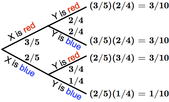
Figure 3. The probability of any outcome (leaf) in a probability tree diagram is given by the product of probabilities from the start of the tree to the outcome. For example, the probability that X is blue and Y is red is equal to (2/5)(1/4), or 1/10.

Two random variables are dependent if they are not independent. For an example of dependent random variables, recall our example in “Mendel's First Law” of drawing two balls from a bag containing 3 red balls and 2 blue balls. If $X$ represents the color of the first ball drawn and $Y$ is the color of the second ball drawn (without replacement), then let $A$ be the event "$X$ is red" and $B$ be the event $Y$ is blue. In this case, the probability tree diagram illustrated in Figure 3 demonstrates that $\mathrm{Pr}(A \textrm{ and } B) = \frac{3}{10}$. Yet we can also see that $\mathrm{Pr}(A) = \frac{3}{5}$ and $\mathrm{Pr}(B) = \frac{3}{10} + \frac{1}{10} = \frac{2}{5}$. We can now see that $\mathrm{Pr}(A \textrm{ and } B) \neq \mathrm{Pr}(A) \times \mathrm{Pr}(B)$.