Dec. 4, 2012, 7:02 a.m. by Rosalind Team
Topics: Heredity, Probability
Introduction to Mendelian Inheritance
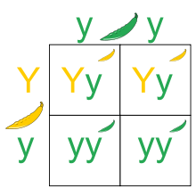
Figure 1. A Punnett square representing the possible outcomes of crossing a heterozygous organism (Yy) with a homozygous recessive organism (yy); here, the dominant allele Y corresponds to yellow pea pods, and the recessive allele y corresponds to green pea pods.Modern laws of inheritance were first described by Gregor Mendel (an Augustinian Friar) in 1865. The contemporary hereditary model, called blending inheritance, stated that an organism must exhibit a blend of its parent's traits. This rule is obviously violated both empirically (consider the huge number of people who are taller than both their parents) and statistically (over time, blended traits would simply blend into the average, severely limiting variation).
Mendel, working with thousands of pea plants, believed that rather than viewing traits as continuous processes, they should instead be divided into discrete building blocks called factors. Furthermore, he proposed that every factor possesses distinct forms, called alleles.
In what has come to be known as his first law (also known as the law of segregation), Mendel stated that every organism possesses a pair of alleles for a given factor. If an individual's two alleles for a given factor are the same, then it is homozygous for the factor; if the alleles differ, then the individual is heterozygous. The first law concludes that for any factor, an organism randomly passes one of its two alleles to each offspring, so that an individual receives one allele from each parent.
Mendel also believed that any factor corresponds to only two possible alleles, the dominant and recessive alleles. An organism only needs to possess one copy of the dominant allele to display the trait represented by the dominant allele. In other words, the only way that an organism can display a trait encoded by a recessive allele is if the individual is homozygous recessive for that factor.
We may encode the dominant allele of a factor by a capital letter (e.g.,
$\mathrm{A}$ ) and the recessive allele by a lower case letter (e.g.,$\mathrm{a}$ ). Because a heterozygous organism can possess a recessive allele without displaying the recessive form of the trait, we henceforth define an organism's genotype to be its precise genetic makeup and its phenotype as the physical manifestation of its underlying traits.The different possibilities describing an individual's inheritance of two alleles from its parents can be represented by a Punnett square; see Figure 1 for an example.
Probability is the mathematical study of randomly occurring phenomena. We will model such a phenomenon with a random variable, which is simply a variable that can take a number of different distinct outcomes depending on the result of an underlying random process.
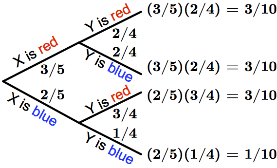
For example, say that we have a bag containing 3 red balls and 2 blue balls.
If we let
Random variables can be combined to yield new random variables. Returning to the ball example,
let
An event is simply a collection of outcomes. Because outcomes are distinct, the probability
of an event can be written as the sum of the probabilities of its constituent outcomes.
For our colored ball example, let
Given: Three positive integers
Return: The probability that two randomly selected mating organisms will produce an individual possessing a dominant allele (and thus displaying the dominant phenotype). Assume that any two organisms can mate.
2 2 2
0.78333
Hint
Consider simulating inheritance on a number of small test cases in order to check your solution.