Glossary

Connectivity in undirected graphs is pretty straightforward: a graph that is not connected can be decomposed in a natural and obvious manner into several connected components. Depth-first search does this handily, with each restart marking a new connected component.

In directed graphs, connectivity is more subtle. In some primitive sense, the directed graph of the following graph is “connected”—it can’t be “pulled apart,” so to speak, without breaking edges. But this notion is hardly interesting or informative. The graph cannot be considered connected, because for instance there is no path from $G$ to $B$ or from $F$ to $A$.

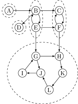
The right way to define connectivity for directed graphs is this: Two nodes $u$ and $v$ of a directed graph are connected if there is a path from $u$ to $v$ and a path from $v$ to $u$. This relation partitions $V$ into disjoint sets that we call strongly connected components. The graph above has five of them.

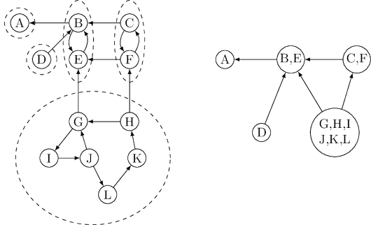
Now shrink each strongly connected component down to a single meta-node, and draw an edge from one meta-node to another if there is an edge (in the same direction) between their respective components. The resulting meta-graph must be a dag. The reason is simple: a cycle containing several strongly connected components would merge them all into a single, strongly connected component. Restated,

Property Every directed graph is a dag of its strongly connected components.

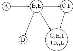
This tells us something important: The connectivity structure of a directed graph is two-tiered. At the top level we have a dag, which is a rather simple structure—for instance, it can be linearized. If we want finer detail, we can look inside one of the nodes of this dag and examine the full-fledged strongly connected component within.

An efficient algorithm

The decomposition of a directed graph into its strongly connected components is very informative and useful. It turns out, fortunately, that it can be found in linear time by making further use of depth-first search. The algorithm is based on some properties we have already seen but which we will now pinpoint more closely.

Property 1 If the ${\tt explore}$ subroutine is started at node $u$, then it will terminate precisely when all nodes reachable from $u$ have been visited.

Therefore, if we call ${\tt explore}$ on a node that lies somewhere in a sink strongly connected component (a strongly connected component that is a sink in the meta-graph), then we will retrieve exactly that component. The graph above has two sink strongly connected components. Starting explore at node $K$, for instance, will completely traverse the larger of them and then stop.

This suggests a way of finding one strongly connected component, but still leaves open two major problems: (A) how do we find a node that we know for sure lies in a sink strongly connected component and (B) how do we continue once this first component has been discovered?

Let’s start with problem (A). There is not an easy, direct way to pick out a node that is guaranteed to lie in a sink strongly connected component. But there is a way to get a node in a source strongly connected component.

Property 2 The node that receives the highest ${\tt post}$ number in a depth-first search must lie in a source strongly connected component.

This follows from the following more general property.

Property 3 If $C$ and $C'$ are strongly connected components, and there is an edge from a node in $C$ to a node in $C'$, then the highest ${\tt post}$ number in $C$ is bigger than the highest ${\tt post}$ number in $C'$.

Proof. In proving Property 3, there are two cases to consider. If the depth-first search visits component $C$ before component $C'$, then clearly all of $C$ and $C'$ will be traversed before the procedure gets stuck (see Property 1). Therefore the first node visited in $C$ will have a higher ${\tt post}$ number than any node of $C$ . On the other hand, if $C'$ gets visited first, then the depth-first search will get stuck after seeing all of $C'$ but before seeing any of $C$, in which case the property follows immediately. ∎

Property 3 can be restated as saying that the strongly connected components can be linearized by arranging them in decreasing order of their highest ${\tt post}$ numbers. This is a generalization of our earlier algorithm for linearizing dags; in a dag, each node is a singleton strongly connected component.

Property 2 helps us find a node in the source strongly connected component of $G$. However, what we need is a node in the sink component. Our means seem to be the opposite of our needs! But consider the reverse graph $G^R$, the same as $G$ but with all edges reversed $G^R$ has exactly the same strongly connected components as $G$ (why?). So, if we do a depth-first search of $G^R$, the node with the highest ${\tt post}$ number will come from a source strongly connected component in $G^R$, which is to say a sink strongly connected component in $G$. We have solved problem (A)!

Onward to problem (B). How do we continue after the first sink component is identified? The solution is also provided by Property 3. Once we have found the first strongly connected component and deleted it from the graph, the node with the highest ${\tt post}$ number among those remaining will belong to a sink strongly connected component of whatever remains of $G$. Therefore we can keep using the ${\tt post}$ numbering from our initial depth-first search on $G^R$ to successively output the second strongly connected component, the third strongly connected component, and so on. The resulting algorithm is this.

1. Run depth-first search on $G^R$.
2. Run the undirected connected components algorithm on $G$, and during the depth-first search, process the vertices in decreasing order of their ${\tt post}$ numbers from step 1.

This algorithm is linear-time, only the constant in the linear term is about twice that of straight depth-first search. (Question: How does one construct an adjacency list representation of $G^R$ in linear time? And how, in linear time, does one order the vertices of $G$ by decreasing ${\tt post}$ values?)

Source: Algorithms by Dasgupta, Papadimitriou, Vazirani. McGraw-Hill. 2006.